The roughness analysis characterizes the surface properties with regard to their texture, bearing performance and fluid retention. The parameters can be categorized in four main section:
Read on for detailed explanation and definition.
Roughness parameters are determined in two or three dimensions. Use self-defined cuts or selected areas within your microscopy data or evaluate entire images and image sequences. Here comes the strength of the dotCube software into play: Working with large data bundles happens easily and fast. The results are inserted into tables and neatly arranged plots. And every result is calculated as exact as always expected from dotCube.
dotCube performs the roughness calculations according to well-known international standards DIN4768, ASME B46.1 and ISO 4287/1 which are stated in our documentation as well as in the roughness control panel. We set trends even beyond the common technical standards: The precision of the subsurface adjustment prior data evaluation of dotCube is still unreached giving exceptional precise results even from tilted and distorted images.
Some parameters depend on the definition of a local maximum and a local minimum. We use the following definition: A pixel is a local maximum if all eight neighboring pixels lie lower and a local minimum if all eight neighboring pixels lie higher, respectively.
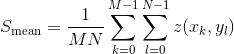
The roughness average,  , is defined as
and the root mean square,  , is
, is
 .
.
The surface skewness,  , measures the asymmetry of the height distribution histogram, and is defined as
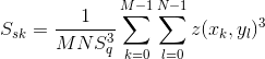 .
.
For symmetric height distribution, e.g. a Gaussian-like height distribution, we find that the Surface Skewness must be equal to zero. If the Surface Skewness is negative, it could be a flat surface with holes and if the Surface Skewness is positive, it could be a flat surface with peaks. If the absolute value of Surface Skewness is greater than one, there could be extreme holes or peaks on the surface.
The surface kurtosis,  , measures the density of topographic peaks on a surface, and is defined by
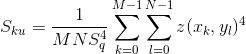 .
.
If we have a Gaussian height distribution, the Surface Kurtosis approaches 3.0 when the number of pixels is increased. The more the value is below 3.0, the wider the height distribution, and vice versa for values that are greater than 3.0.
The peak peak,  , is the height difference between the highest and the lowest pixel on the surface, that is
 ,
,
where  and
and  .
.
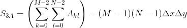
The ten point peak,  , is the sum of the average five highest and average five lowest values of an image:
where  is the
  th highest local maximum and
  is the th lowest local minimum. In the case that there are less than five valid local maximums or five local minimums, the parameter is undefined.
The maximum valley depth indicates the lowest height value of the image meaning the value of the deepest valley:
 .
.
The maximum peak height declares the maximum height value of an image meaning the value of the largest peak:
 .
.
The mean value,  , gives the average height value of the image:
 .
.
There are three hybrid parameters which reflect changes in the amplitude and in the spacing of topography. Their calculations are based on the local z-slopes.
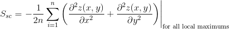
The mean summit curvature,  , describes the average curvature of local maxima:
 .
.
The root mean square gradient,  , states the RMS-value of the surface slope:
 .
.
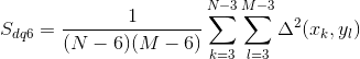
The area root mean square slope,  , is similar to the root mean square gradient but takes more neighbor pixels in the computation of the slope for every pixel into account:
 ,
,
where

 .
.
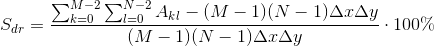
The surfaces area ratio,  , compares the surface area against the area of the xy-plane, and is defined to be
 ,
,
where

 .
.
If we have a totally flat surface, the surface area and the area of the xy-plane are equal and the surfaces area ratio is 0%.
The projected area,  , indicates the area of the flat xy-plane as follows:
 .
.
The surface area,  , is the area of the surface area taking the z height into consideration and is defined as:
 .
.
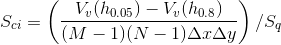
The surface bearing index,  , is defined as
 ,
,
where  means the distance from the top of the surface to the height at 5% bearing area. If the height distribution is Gaussian-like, the surface bearing index is approximately 0.608 for a large number of pixels. Furthermore, a large surface bearing index is a desirable bearing property.
The core fluid retention index,  , is defined via
 ,
,
where  indicates the void area over the bearing area ratio curve and under the horizontal line
  . If the height distribution is Gaussian like, is approximately 1.56 for a large number of pixels. If the values of are large, the volume of air in the core zone is large. For any surface is between 0 and
  .
.
The valley fluid retention index,  , is defined as
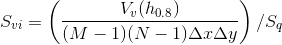 .
.
In the special case of a Gaussian height distribution, the valley fluid retention index approaches 0.11 for increasing numbers of pixels. The meaning of large values of is that the volume of air in the valley zone is big. For any surface the value of is between zero and 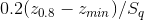 .
.
The spatial properties consist of the density of summits, texture direction, dominating wavelength and index parameters. The density of summits is computed in the spatial domain from the image while the others rely on the Fourier spectrum in the frequency domain.
The density of summits,  , is the number of local maximums per area:
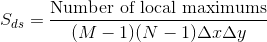 .
.
Since the parameter is sensitive to noise, it should be treated with caution.
The texture direction,  , is defined as the angle of the dominant texture direction in the image. If the image is composed of parallel ridges, the texture direction is parallel to the direction of the ridges. If the ridges are perpendicular to the X-scan direction, the texture direction is precisely zero. If the angle of the ridges is rotated clockwise, the angle is positive, and if the angle of the ridges is rotated counterclockwise, the angle is negative. This parameter provides interesting information only if a dominant direction exists.
The texture direction is calculated from the Fourier spectrum. The relative amplitude for various angles is found by their amplitude's summation along M equidistant radial lines resulting in the angular spectrum. The amplitude sum,  , for a line with the angle
  is defined as
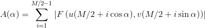 .
.
The angle with the highest amplitude sum  is the dominant direction in the Fourier transformed image and perpendicular to the direction of the texture.
The texture direction index,  , specifies how dominant the predominating texture is and is defined as
 .
.
With this definition, the texture direction index is always between zero and one. A low index indicates a strongly dominant texture while a value close to one describes evenly distributed texture directions.
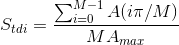
The radial wavelength,  , is the dominating wavelength in the radial spectrum. The radial spectrum is calculated by summation of the amplitude values around the M/2 - 1 equidistant half circles. The radius is measured in pixels of the half circles, r, is
  . The amplitude sum, B(r), along a half circle with the radius r, is
 .
.