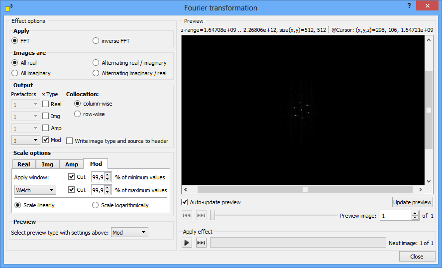
The Fourier transform is a powerful tool for analyzing wavelike or periodic structures. DotCube offers the fast Fourier transform as well as the inverse Fourier transform. Select the kind of your input data - real or imaginary - as well as the output presets and arrangements. Choose a window function and an applicable scaling of the z axis. The Fourier transform function will generate new transformed images and arrange them according to your settings.
For further details see the extensive explanation:
Forward or inverse Fourier transformation
DotCube offers the Fourier transformation in both directions. Select one of the "FFT" or "inverse FFT" options.
The images might be real or imaginary data. Choose the appropriate option:
Option |
Description |
All real |
All input images contain real data. |
All imaginary |
All input images contain imaginary data. |
Alternating real / imaginary |
The input image stack contains periodically initially a real data image followed by an imaginary one. |
Alternating imaginary / real |
The input image stack contains periodically initially a imaginary data image followed by a real one. |
If you select one of the "Alternating..." options, at least two images should be available. Otherwise an error message is displayed. In this case of odd numbers, the last image will be ignored.
In the output group box, one or multiple kinds of transforms can be selected by checking the "Real", "Img", "Amp" and "Mod" options with prefactor presets.
The available targets are:
Option |
Description |
Real |
The target contains only the real data part. |
Img |
The target contains only the imaginary data part. |
Amp |
The target contains the absolute values of the real data part. |
Mod |
The target contains the vector length |
To simplify working with large data bundles, the input images will be arranged in vertical or horizontal order. Two default collocation settings are available. The "column-wise" option will arrange the input images in a vertical order and any new output images column-wise. The "row-wise" option will put the input images in a horizontal order and arrange any new output images row-wise.
For later analysis, the Fourier function supports writing the settings and the source image names to the output image header. Select the "Write image type and source to header" option if applicable.
The scale options group box enables you to
Data which is not finite periodic will cause artifacts in the Fourier transforms. Therefore, window function may be applied to suppress artifacts and enhance the visibility of the main spots. DotCube offers seven most common window functions w(x). Their behavior in real space is explained in the table below:
Window |
Function |
Rectangular |
"0.5" at image borders, "1" elsewhere |
Hann |
w(x) = 0.5 - 0.5⋅cos(2πx) |
Hamming |
w(x) = 0.54 - 0.46⋅cos(2πx) |
Blackmann |
w(x) = 0.42 - 0.5⋅cos(2πx) + 0.08⋅cos(4πx) |
Welch |
w(x) = 4x⋅(1 - x) |
Nutall |
w(x) = 0.355768 - 0.487396⋅cos(2πx) + 0.144232⋅cos(4πx) - 0.012604⋅cos(6πx) |
Flattop |
w(x) = 0.25 - 0.4825⋅cos(2πx) + 0.3225⋅cos(4πx) - 0.097⋅cos(6πx) + 0.008⋅cos(8πx) |
If applicable, you might cut all values below a lower limit (infimum) or above an upper limit (supremum). The cut values are set to the average z value. To cut the extreme values emphasis the main Fourier spots. Cutting as much values as possible leads to best Fourier spot results.
In linear scale the Fourier spots might be poorly visible. Select the "Scale linearly" or "Scale logarithmically" to define the scaling of the z axis.
The preview window displays only one possible Fourier transform. Select your favorite transform to preview in this group box.
The execution of the function may be started by pressing two different shortcut keys:
For more shortcut keys see our detailed list.