The possibility of identifying, analyzing and tracking structures and objects is probably the central feature of the dotCube project. This is done via a rich function library which will enable you to analyze structures in great detail and track data in a dependable and time-efficient manner. Once a structure has been identified, the structure itself and the changes that occurred to it can be tracked across multiple images.
Read on for getting to know in detail about:
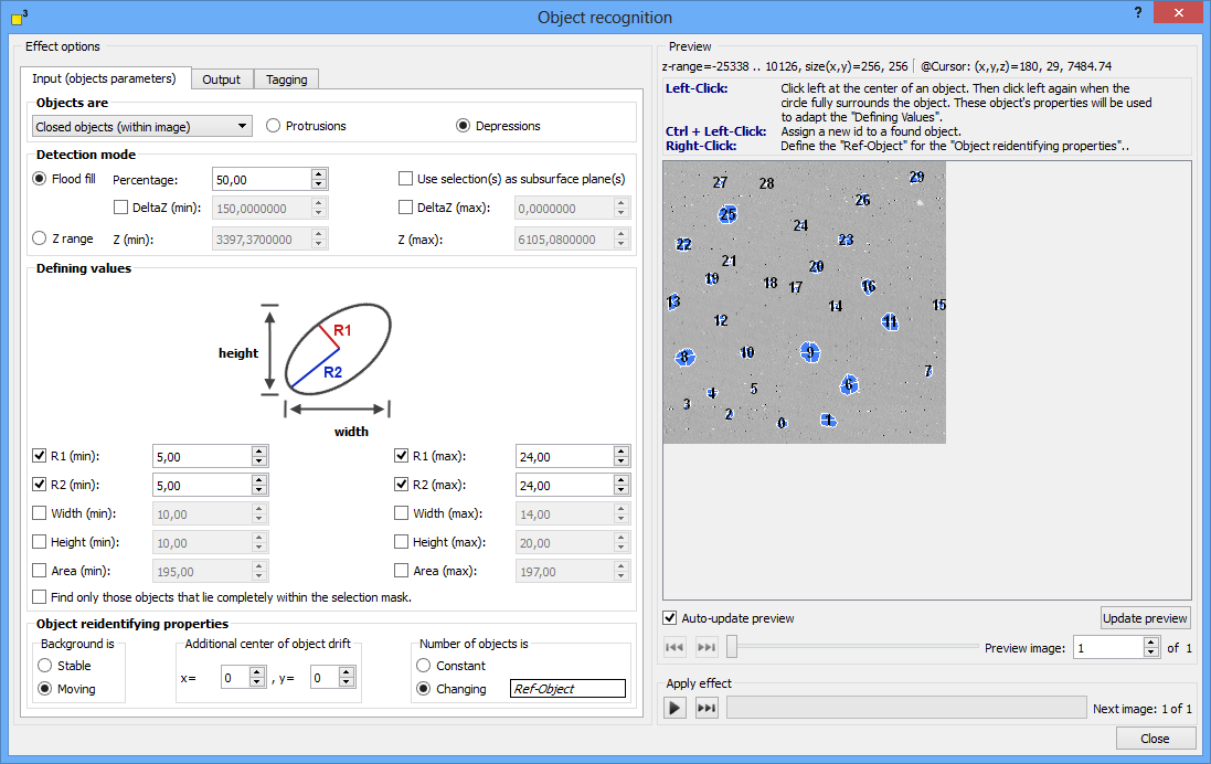
The object recognition dialog is designed to speed up the analysis process. Therefore, the most common used control elements are placed on the first "Input parameters" page in the tabulator view. The input parameters define structural requirements, which help to identify user-demanded valid objects.
For starting the analysis process, define
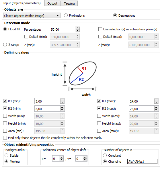
The fundamental properties are defined in the "Objects are..." group box.

Select the physical border appearance of your favorite objects:
Property |
Description |
Closed objects |
The border of the objects proceeds continuously and is not broken by the image boundaries (e.g. an elliptical shape). |
Open objects |
The object border is broken up (e.g. an half circular object bordering at the image boundaries). |
Open and closed objects |
All objects are valid regardless of their border progression. |
Specify if your wanted objects are valley-like depressions or mountain-like protrusions by selecting the applicable option "Depression" or "Protrusion".
The more precise geometric properties are defined in the "Defining values" group box.
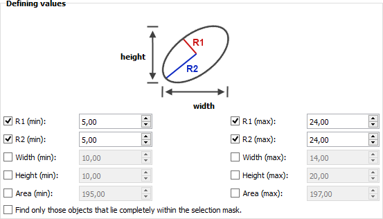
Select any properties which define your favored objects best and specify their values. If you are looking for regular shaped structures, use the radius options. For irregular or dentritic shapes, width and height are a better choice. The smaller the minimum values are, the more computing time will be used by the search algorithms. But the time consumption is crucial only by selected "flood fill mode". The "Z range mode" algorithm is much faster.
If the selected geometric properties are not sufficient, an error message will be displayed.
If you need assistance for defining the geometric input values, click on an object of your interest and move the mouse to its border and further onto the surrounding area. The dotCube assistant spans a circle around the clicked position. If the object is fully encircled, click again and the dotCube assistant will suggest a reasonable geometric parameter set.
Depending on the kind of your data, two complementary algorithms are available:
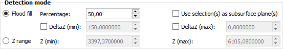
The flood fill algorithm demands more computing time, but delivers accurate and reliable results even with noisy and slightly distorted image data. Objects are identified by their height differences to their local environment. Thus, the results are highly precise.
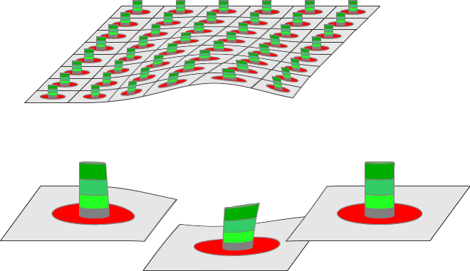
The image above shows a schematic drawing with green objects on a gray surface. The flood fill algorithm compares every possible object candidate with its local surrounding height level marked in red. Hence, the green objects are found independently from the curvature of the surface.
The fill "Percentage" value specifies the minimum height difference between the surrounding surface and the object pixels. A low "Percentage" value will assign only data points with a large height difference to an object (the greenest parts of the sketched objects). The higher the value the smaller the height limitations are. In the upper limit ("Percentage" = 100%) an height limit between surface and object does not exist. But then, no objects would be identified, because the geometric defining restrictions will be exceeded and therefore violated.
Although the flood fill algorithm is heavily robust, the surrounding height calculations might fail in strongly distorted images. In these cases, you may mark manually several surface regions as reference heights. The reference height which is closest to each object height will be used.
In addition to the "Percentage" value, there is the possibility to add distinct constant height limits which are dispensable for some special analysis processes. If all of the conditions above are fulfilled, but the height difference between object pixel and subsurface is less than the "Delta z(min)" value and the "Delta z(min)" optional condition is activated, the object will be discarded. If the "Delta z(max)" option is selected, any object which exceeds the height difference between itself and the surface named in "Delta z(max)" will be discarded.
Let's have a look at an example: We would like to analyze an image, but want to exclude any object, which is less than 10nm higher than its surroundings. Therefore, we would select the "Delta z(min)" option and set its value to "10" if nanometers are the natural unit of your image.
The "Z range mode" works much faster than the flood fill mode, but uses only one height range for each object. Any object featuring an height within the specified "Z (min)" and "Z (max)" range is a valid object and will be found dependent on the defining geometric properties. While this tool is very helpful for searching objects within a absolute distinct height level, a tilted or curved image might causes misleading object results in the "Z range mode". In unfavorable cases, the results might be incomplete objects or artifacts.
The output parameters section offers to you a rich selection of feasible properties which can be calculated and displayed in the table section, written into each image header or drawn on the picture layer. Furthermore, the draw settings and the selected objects in the object filter and the filter presets can be changed.
Computing results - the output selection dialog
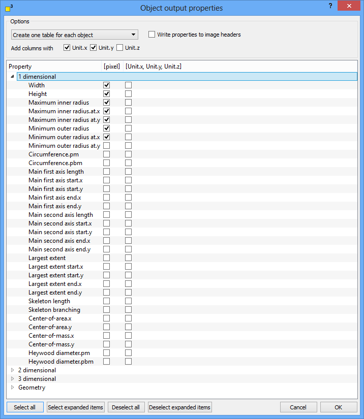
The object output properties dialog provides the numerical output options of the object recognition function. Select
There are four table output options available:
Option |
Description |
Create one table for each object |
For any object in any selected image, a new table is created and filled. E.g.: If one or several images contain an object with the id "3", one new table will be created and filled with object properties of object 3. |
Create one table for each image |
For any image, a new table is created and the properties of any object in one single image are filled in. E.g.: If you analyze five images, five new tables will be created and they will be filled with properties of any object which was found in each currently analyzed image. |
Create one table for all |
Only one new table is created and all object properties are filled in. |
Add results to current table if appropriate |
This option adds every future analysis to the current table if the numbers and titles of table columns fit. |
No table output |
No tabular output is displayed. |
If you decide to display the object properties in natural units, you might supplementary add one, two or three columns with the natural units of the x, y and z dimensions. Therefore, select the appropriate "unit" check boxes.
All computed object properties might be added to the image header for further analysis. Select the "Write properties to image headers" option to do so. The "Edit object" tool, a member of the scientific tool bar, enables you at any time to list all object properties from the image headers or the object layer into tables.
DotCube provides an extensive selection of object properties which can be calculated. They are sorted by one dimensional, two dimensional, three dimensional and geometric headlines. Select your favorite properties and if you want them to be displayed in natural units or in pixels. Use the "Select all", "Select expanded items" as well as "Deselect all" and "Deselect expanded items" buttons to speed up the selection process.
Read on for detailed explanation of every computable property.
Returns the expansion in x direction.
Returns the expansion in y direction.
Calculates the radius of the in-circle.
Calculates the radius of the perimeter.
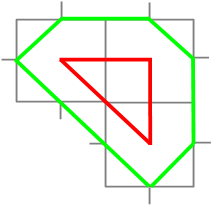
Numerical sciences provide a large variety of methods for calculating circumferences of discrete data. DotCube offers two complimentary methods called "pm" and "pbm" outlined in the scheme below. The object pixels are gray colored. The "pm" result is displayed in red color, the "pbm" result in green color:
The main axes section determines the two main directions of the area moment of inertia. DotCube provides their crossing points with the object borders and each axis length.
Returns the maximum distance of any object pixel.
The skeleton of an object is determined by the algorithm of T.Y. Zhang and C.Y. Suen described in their publication "A fast parallel algorithm for thinning digital patterns" and published in "Communication of the ACM" (volume 27 number 3). Thereby, the object expansion is shrinked until it exhibits single lines which are called branches. During this process, the deletion of branch endings is nearly but not completely suppressed preserving the origin object length.
The property "Skeleton length" designates the most extensive length of the skeleton. "Skeleton branching" labels the number of branch endings.
E.g.: If you analyze the shape of a worm like structure, the skeleton length names the length of the worm and the skeleton branching will give the value "2" because the worm features two endings.
Denotes the centroid of the object area.
Labels the x- and y coordinates of the centroid of the object volume.
Designates the equivalent diameter to a circular area. Two different heywood diameters can be calculated ("pm" and "pbm") because there are two different methods to calculate area values depending on its borders (see also circumference calculation).
![]()
The area denotes the number of pixels which are occupied by an object. Due to the discrete character of the data, two different options for rating the border pixels are available: "pm" and "pbm". See circumference calculation for further explanation.
The bounding box declares a rectangular frame which belts the object pixels without touching any of them. The left-top and right-bottom positions are calculated.
Cubage characterizes the volume of an object and is defined as the height difference between every object pixel and the object surrounding surface. The total sum of the entire height differences gives the cubage value.
The object minimum labels the object pixel with the smallest height. The x-, y- and z coordinates are available.
The object maximum names the object pixel with the largest height. The x-, y- and z coordinates are available.
The object mean designates the average height of the entire object.
The object range names the z range of the object. The range is calculated by subtracting the minimum object height value from the maximum object height value.
The object standard deviation labels the standard deviation of the height values of an object.
The border minimum labels the border pixel with the smallest height. The x-, y- and z coordinates are available.
The border maximum names the border pixel with the largest height. The x-, y- and z coordinates are available.
The border mean designates the average height of the object border.
The border range names the z range of the object border. The range is calculated by subtracting the minimum object border height value from the maximum object border height value.
The border standard deviation labels the standard deviation of the height values of the object's border.
The aspect ratio denotes the relation between the two main axes. The ratio is given by the length of the main first axis divided by the length of the main second axis.
The compactness characterizes how much the shape of an object differs from a circle. A circle is defined by the value "1", less circular objects are rated with higher values.
The definition of compactness is given by
![]() .
.
The fractal dimension denotes the dimension of structures with non integer values. While rectangles and cubes exhibit integer dimensions "1" respectively "2", fractals feature dimensional values in between.
The fractal dimension is calculated by the box counting method. Therefore, the object is superposed by a grid. All grid elements which are occupied by object pixels are counted. The limit of the logarithmic relation between occupied grid elements N and their edge length ε gives the fractal dimension value:
![]() .
.
The elongation characterizes the shape of an object. The more circular an object is shaped, the more the elongation converge towards zero. More elongated structures like rectangles will get values converging towards "1".
The orientation labels the angle between the x direction and the first main axis.
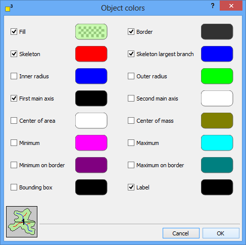
The color and labeling chapter describes the settings for visualizing the analyzed data.
Click on the "Colors" button on the output page in the tabulator view to select which object properties should be drawn and select their color. An example is provided on the left bottom in the colors dialog. For detailed explanation of the properties see the output values section.
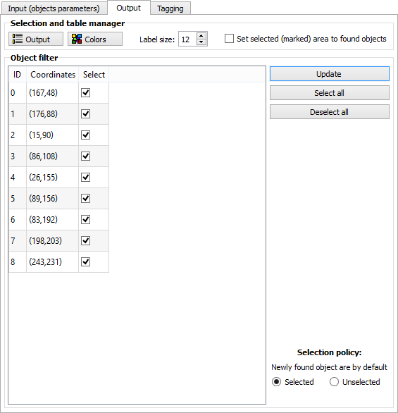
dotCube will allocate a unique numeric identification number ("ID") to every found object. You might modify the
The label size can be changed on the output page of the tabulator view in the "Selection and table manager" section (see image below).

To modify the label color or switch on/off the drawing of the labels, click on the "Colors" button. For further explanation, see the colors section.
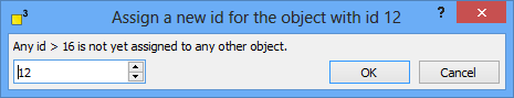
The IDs are allocated automatically by the object recognition function and its tracking settings. If you want to change the IDs, press CTRL and click on the object. The ID change dialog (see image below) will open and give you a hint which IDs are still not assigned. You might choose both, an unoccupied or an already assigned ID. In the second case, your object will get the demanded ID and the object which had this very ID previously will get the next unoccupied one.
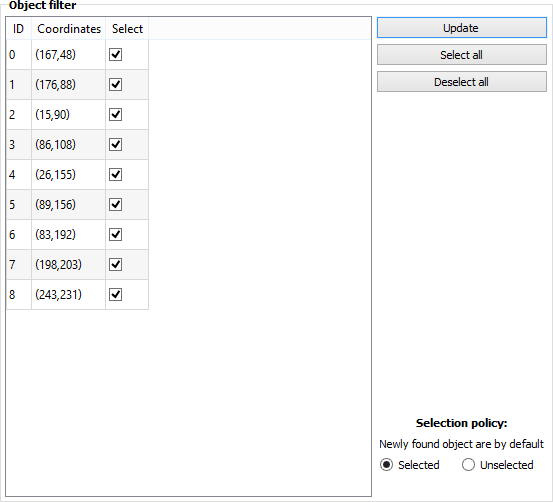
The object filter assists you to concentrate on interesting features and neglect uninteresting objects. Every found object is filled into the filter list with its ID and centroid coordinates. Select any object which should be analyzed. Use the "Select all" and "Deselect all" buttons if applicable. Only the properties of selected objects are drawn and filled into tables and image headers.
Attention: Please note that any unselected object will not be displayed in the preview. If you cannot find your favorite objects, check the selection status in the filter list. Furthermore, read carefully the "Selection policy" section.
To enable fast analysis processes dotCube has a special built-in selection policy for
The selection presets for newly found objects can be modified by changing the options "Selection policy for following images" from selected to unselected status and vice versa. If you have chosen "unselected", objects which were not found in the previous image or preview will be unselected and therefore invisible. Choose "selected" if you would like to display any newly found objects.
Tracked objects are objects with the same ID in the previous image or preview. Their selection status will be transferred to the current image no matter which selection presets you had chosen. To modify their visibility and their analysis status, you have to change their selection status manually in the object filter.
The dotCube built-in tracking options force the pace of analysis processes dramatically. After selecting the objects of your interest in the first image, they are tracked in consecutive images and their data is sorted and filled in tables exactly how you need it.
According to the concept of dotCube, we provide an automatic and robust function with the chance to arrange adjustments manually. Modify the automatic tracking settings in the tracking parameters and adjust the results by manual tagging.
The tracking algorithm has to distinguish between background drift and object drift. If your objects
do not move in respect to the background, select the "Background is stable" option. Otherwise, select the "Background is moving" option.
The objects in the currently analyzed image are searched within an area range corresponding to their centroid position in the previous image and their expansion. Extent this range by choosing "additional center of object drift" in x and y direction.
If the number of objects which could be found is constant (should be rare), choose the "Number of objects is constant" option. In all other cases, select the "Changing" option.
The case "Moving background" and "Changing object numbers" is the case with the most variability. If you want to make sure that the objects will be re-identified correctly, mark an reference object by right-clicking on an object. This object will get the same ID in the entire analysis process and every other object will be re-identified in respect to this reference object. The coordinates are written in the box with the headline "Ref-Object". After a reference is marked, the previously red colored "Ref-Object" box will be re-colorized in green. To correct your reference choice, just right click again. Only the last reference click per image is evaluated.
![]()
The manual tagging page is intended to assist you during manual tracking adjustments. On the left side, you see the previously analyzed image with the found objects. On the right side, the currently analyzed image with its objects is displayed. To change an object ID, press CTRL and left-click on an object (on Apple systems: Apple key and left-click). For further details, see the change labels section.
The execution of the function may be started by pressing two different shortcut keys:
For more shortcut keys see our detailed list.